Aerospike is known for incredible speed and scalability. As a bonus, people using Aerospike often recognize a far lower Total Cost of Ownership (TCO) compared with other technologies. Optimizing the distribution of data between servers contributes to this low TCO and Aerospike's uniform balance feature allows for almost-perfect even distribution of data across the servers, resulting in better resource utilization and easier capacity planning. This blog post examines how this feature works.
Clustering
To fully understand the benefits of how uniform balance works, let's start by reviewing the normal Aerospike partitioning scheme.
In Aerospike, each node in a cluster must have an ID. This can be allocated through the node-id configuration parameter, or the system will allocate one, but every node must have a distinct ID. For this explanation, assume there is a 4 node cluster with node-ids of A, B, C, D.
When the cluster forms, once all members agree that they can see all other nodes, a deterministic algorithm runs to form a partition map. Aerospike has 4096 partitions, and the partition map dictates how these partitions are assigned to nodes. For example, a normal partition table might look something like this:
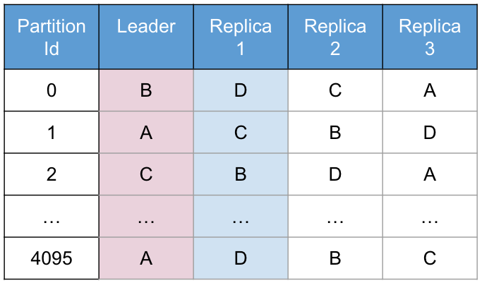
Figure 1: Partition Table with RF = 2 and 4 nodes
Forming the partition table
The algorithm used to form this table is fairly simple. The partition ID is appended to the node ID, then hashed and the results sorted. For example, for partition 1 in this table we might have:
hash("A:1") => 12
hash("B:1") => 96
hash("C:1") => 43
hash("D:1") => 120
sort({12, "A:1"}, {96, "B:1"}, {43, "C:1"}, {120, "D:1"})
  => {12, "A:1"}, {43, "C:1"}, {96, "B:1"}, {120, "D:1}
Hence node A would be the leader for partition 1, followed by C then B then D. With 2 copies of the data (replication factor = 2), A is the leader and C is the replica.
This algorithm is applied across all 4096 partitions to form the partition table. This is a deterministic algorithm - the same 4 node-ids will always form the same partition table.
Partitioning design goal
When this partitioning algorithm was created, the goal was to minimize data movement in the event of a node loss or addition. For example, consider what happens if node C fails. All the nodes in the cluster are sending heartbeats to one another and after a number of missed heartbeats (controlled by the timeout configuration parameter in the heartbeat section of the configuration file), the node is considered "dead" and ejected from the cluster.
Immediately after this, the cluster creates a new partition map using the above algorithm, but without C in it. Given the sorting, the effect this has in practice is to "close" the holes left by the removal of C by shifting everything which was to the right of C in the table, one place to the left.
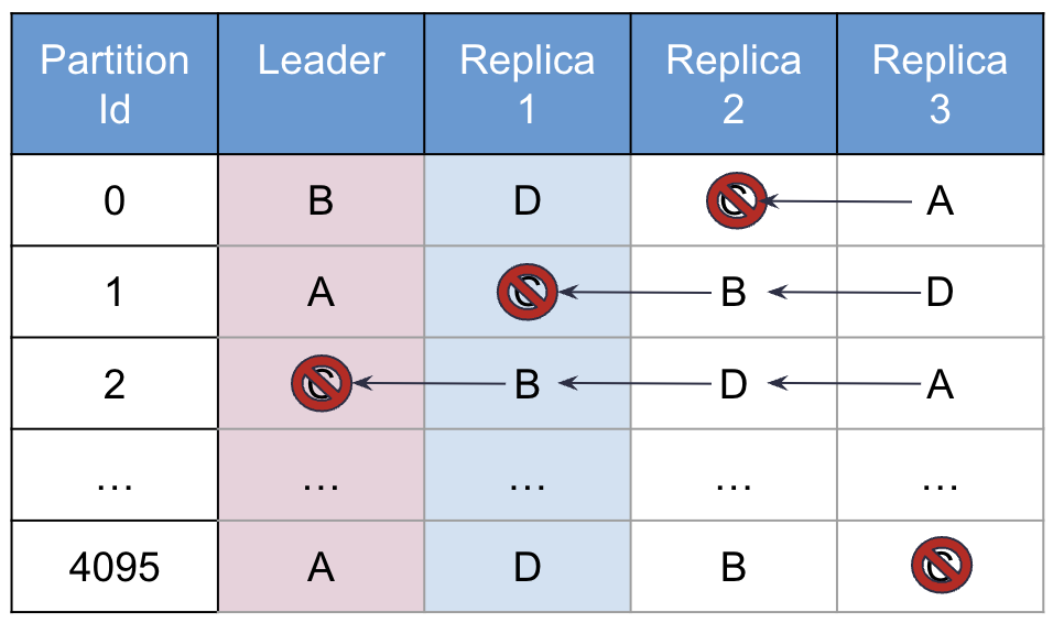
Figure 2: Partition Table after Node C has been removed
As Figure 2 shows, the only affected partitions to cause data movement are where C was either the leader or the replica, with these results:
On partition 1, C was the replica and B is promoted to replica with A migrating a copy of the data to B.
On partition 2, C was the leader, so B is promoted to leader (no data movement necessary as it has a full copy of the data) and D is promoted to replica. B migrates a copy of the data onto D.
On partitions 0 and 4095, no data movement is necessary as C was neither a leader or replica.
Should C be added back into the cluster, it returns to its previous location in the partition map, again minimizing the amount of data required to be migrated. Additionally, if a new node E is introduced to the cluster, only partitions where E is either the leader or the replica will require data migrations.
Issue with Design
This algorithm clearly minimizes the amount of data which is migrated between nodes in the case of node removal or addition. However, this is not always optimal from a data volume perspective. Consider a simplified partition map with just 4 partitions in it:
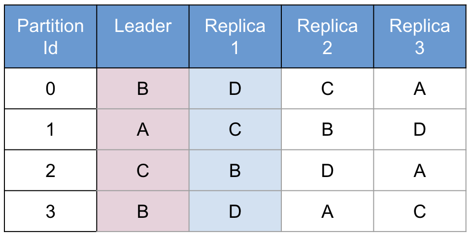
Figure 3: Unbalanced Partition Table
The hashing algorithm described in Figure 3 could easily produce a table like this. This is unbalanced:
Node | Leader Partitions | Follower Partitions | Total Partitions |
A | 1 | 0 | 1 |
B | 2 | 1 | 3 |
C | 1 | 1 | 2 |
D | 0 | 2 | 2 |
This particular distribution highlights 2 problems:
Data volume inconsistency : Node A contains 1 partition, node B contains 3 partitions, so node B will have about 3x the data volume of node A. This can make capacity planning very difficult.
Processing load inconsistency : Aerospike reads and writes from the leader node by default. Writes are replicated by the leader to the follower, but in most cases all reads are served by the leader. So for writes in this example, node B will be involved as a leader or replica on 3 partitions (0, 2, 3) but node A will only be involved on 1 partition (1). The result is that node B will be processing about 3 times as much write traffic as node A. For read traffic, node B will serve traffic from 2 partitions (0, 3) but node D is the leader of no partitions and hence will serve no read traffic.
This is a contrived example based on only 4 partitions. In practice, the larger number of partitions Aerospike uses (4096) will smooth this out to some degree, but production customers still saw variances in the nodes in their cluster of up to 50%.
Uniform balance
This variance between nodes, both in data volume and processing requests, caused difficulty in capacity planning and node optimization. Aerospike clusters typically have homogeneous nodes with regard to processors, network, memory and storage, so having a heterogeneous distribution of partitions to nodes can result in sub-optimal configurations.
The solution, introduced in Aerospike Enterprise version 4.3.0.2 was to tweak the algorithm. The majority of the partition table still follows the algorithm, but the last 128 partitions are tweaked to even out the number of leader partitions each node has. Consider the contrived table again, with the last row tweaked:
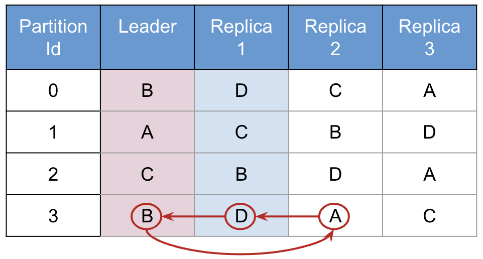
Figure 4: Tweaking the Algorithm
If this table were tweaked in this fashion, every node would end up being the leader of 1 partition and the replica of 1 partition - an optimal distribution. Note that the algorithm doesn't guarantee that the replicas will be perfectly balanced, however they typically are.
The tweaking of the last 128 rows in real Aerospike clustering is again done in a deterministic manner, meaning that each node can compute the partition table independently. The same invariant is true: when a node leaves and re-enters the cluster, it will appear in the same location in the partition map for each partition. However, due to this tweaking it is possible that more data might have to be migrated than before on these last 128 partitions. In practice, this extra data migration is small and the benefits of even partition distribution typically far outweighs this extra network cost.
Note that clusters with rack awareness enabled might experience higher migrations under prefer-uniform-balance. For more information, see this support article about expected migrations after node removal and How does Rack Aware and Prefer Uniform Balance interact.
The prefer-uniform-balance configuration flag dictates whether this tweak to the partitioning algorithm is enabled or disabled. This is an Enterprise Edition feature only, the Community Edition behaves as described above without tweaking the last 128 rows.
Actual Results
Testing a complex algorithm like this is good in controlled conditions, but the real proof comes when implemented by customers. One customer with a large, multi-node cluster was kind enough to send us a screenshot of the transactions per second (TPS) per node of a production cluster showing the period when prefer-uniform-balance was set to true:
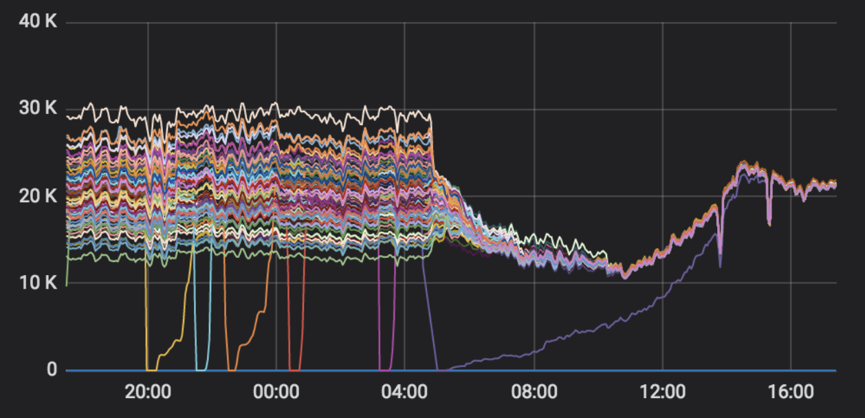
Multi-node cluster before and after turning on prefer-uniform-balance
As you can see, the initial state had a wide variance of TPS between the nodes, ranging from ~15k TPS to ~30k TPS. Once prefer-uniform-balance was enabled, this quiesced to a steady state with all nodes around the same level of ~22k TPS, and less than a 5% variance per node. (Note that node maintenance was going on when this graph was captured, resulting in some nodes having no TPS for short periods of time).
The results from customer deployments of the uniform balance algorithm are so effective, and the down-sides so minimal that prefer-uniform-balance was defaulted to true in Aerospike Server version 4.7.